Using RStudio as an interactive GIS with Leaflet

• Web: http://personal.tcu.edu/kylewalker
• Twitter: https://twitter.com/kyle_e_walker

For exploratory GIS work, I have hesitated to use R instead of ArcGIS or QGIS due to a lack of visual interactivity. One of the things I have appreciated about desktop GIS software is its ability to run a function and then show the results in an interactive data view that I can zoom and pan around. However, with the new Leaflet package for R by RStudio, I can use RStudio in this way for exploratory GIS.

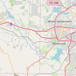
I’ve put together a few examples to show my GIS students at TCU, and I thought I’d share how I created them to demonstrate the interactive GIS functionality that is now in RStudio. For my example, I’ll be doing some GIS operations with the open Starbucks dataset, which you’ll need to download from the link if you want to reproduce this. I’ll look specifically at Starbucks in my city, Fort Worth. In a real analysis, you’d want to use Starbucks locations in the Fort Worth suburbs as well (as the city of Fort Worth has a very odd shape) but this will work as an example.

To get started, I’ll load in the required libraries and the data. I’ll create a SpatialPointsDataFrame from my Starbucks data frame, and then project the data to an appropriate projected coordinate system for buffering (UTM Zone 14N) with the spTransform function.

library(leaflet)
library(rgeos)
library(rgdal)
library(spatstat)
library(maptools)

starbucks <- read.csv('starbucks.csv')

fw <- subset(starbucks, City == 'Fort Worth')

coords <- cbind(fw$Longitude, fw$Latitude)

## Spatial points w/the WGS84 datum

sp_fw <- SpatialPointsDataFrame(coords = coords, data = fw, proj4string = CRS("+proj=longlat +datum=WGS84"))

sp_fw_proj <- spTransform(sp_fw, CRS("+init=epsg:26914"))

For the first example, I’ll create 2km buffers with the gBuffer function from the rgeos package around each Starbucks location. To show the data on a Leaflet map, I’ll need to convert back to using XY coordinates so that the Leaflet package can read it in. The map will show Starbucks locations with markers and a pop-up, the buffers, and the default OSM basemap, and appear right in your RStudio viewer.

buff2km <- gBuffer(sp_fw_proj, byid = TRUE, width = 2000)

buff_xy <- spTransform(buff2km, CRS("+proj=longlat +datum=WGS84"))


leaflet() %>%
  addMarkers(data = fw, 
             lat = ~ Latitude, 
             lng = ~ Longitude, 
             popup = fw$Name) %>%
  addPolygons(data = buff_xy, color = "green", fill = "green") %>%
  addTiles()

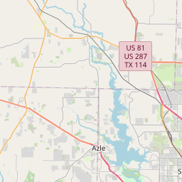
There are many other types of operations we can do. Here, I’ll draw a convex hull around the points:

hull <- gConvexHull(sp_fw_proj)

hull_xy <- spTransform(hull, CRS("+proj=longlat +datum=WGS84"))


leaflet() %>%
  addMarkers(data = fw, 
             lat = ~ Latitude, 
             lng = ~ Longitude, 
             popup = fw$Name) %>%
  addPolygons(data = hull_xy, color = "green", fill = "green") %>%
  addTiles()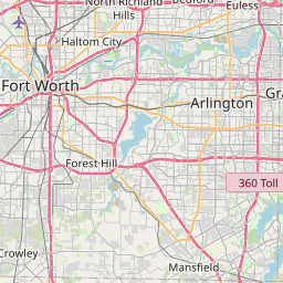

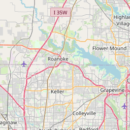
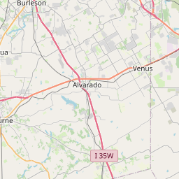
Now, let’s try something a little more complicated. I’m going to draw Thiessen (or Voronoi, Dirichlet) polygons around each point. Each Thiessen polygon represents the area that is nearest to the point that it contains for a given study area (window in the code below). After a bit of StackOverflowing I was able to get this done with help from the spatstat package. I’m setting this up so that each polygon has a popup as well that shows its area in square kilometers.

fw_coords <- sp_fw_proj@coords

## Create the window for the polygons

window <- owin(range(fw_coords[,1]), range(fw_coords[,2]))

## Create the polygons

d <- dirichlet(as.ppp(fw_coords, window))

## Convert to a SpatialPolygonsDataFrame and calculate an "area" field.  

dsp <- as(d, "SpatialPolygons")

dsp_df <- SpatialPolygonsDataFrame(dsp, 
                                   data = data.frame(id = 1:length(dsp@polygons)))

proj4string(dsp_df) <- CRS("+init=epsg:26914")

dsp_df$area <- round((gArea(dsp_df, byid = TRUE) / 1000000), 1)

dsp_xy <- spTransform(dsp_df, CRS("+proj=longlat +datum=WGS84"))

## Map it!

leaflet() %>%
  addMarkers(data = fw, 
             lat = ~ Latitude, 
             lng = ~ Longitude, 
             popup = fw$Name) %>%
  addPolygons(data = dsp_xy, 
              color = "green", 
              fill = "green", 
              popup = paste0("Area: ", 
                             as.character(dsp_xy$area), 
                             " square km")) %>%
  addTiles()

Of course, if I want to do this again for another place, it is a good idea to wrap this code in a function so you don’t have to write the code over and over. I’ve written a function to create Thiessen polygons as in the above example, but with a different dataset as input. You can view the code at this GitHub Gist.

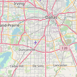
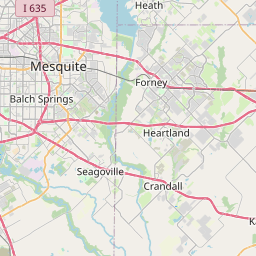
Let’s try it here for Dallas this time:

dallas <- subset(starbucks, City == "Dallas" & State == "TX")

devtools::source_gist(id = "c3c481e566c35ff1d3cd")

leaflet_thiessen(dallas, id = "Name", long = "Longitude", lat = "Latitude", epsg_code = 26914)

Now, with the Leaflet package for R, RStudio can function much better for exploratory GIS work. I look forward to testing this out further!