Preliminaries
Model Formulae
If you haven’t yet read the tutorial on Model Formulae, now would be a good time!
Statistical Modeling
There is not space in this tutorial, and probably not on this server, to cover the complex issue of statistical modeling. For an excellent discussion, I refer you to Chapter 9 of Crawley (2007).
Here I will restrict myself to a discussion of linear modeling. However, transforming variables to make them linear (see Simple Nonlinear Correlation and Regression) is straightforward, and a model including interaction terms is as easily created as it is to change plus signs to asterisks. (If you don’t know what I’m talking about, read the Model Formulae tutorial.) R also includes a wealth of tools for more complex modeling, among them…
- glm( ) for generalized linear models (covered in another tutorial)
- gam( ) for generalized additive models
- lme( ) and lmer( ) for linear mixed-effects models
- nls( ) and nlme( ) for nonlinear models
- and I’m sure there are others I’m leaving out
My familiarity with these functions is “less than thorough” (!), so I shall refrain from mentioning them further.
Warning: an opinion follows! I am very much opposed to the current common practice in the social sciences (and education) of “letting the software decide” what statistical model is best. Statistical software is an assistant, not a master. It should remain in the hands of the researcher or data analyst which variables are retained in the model and which are excluded. Hopefully, these decisions will be based on a thorough knowledge of the phenomenon being modeled. Therefore, I will not discuss techniques such as stepwise regression or hierarchical regression here. Stepwise regression is implemented in R (see below for a VERY brief mention), and hierarchical regression (SPSS-like) can easily enough be done, although it is not automated (that I am aware of). The basic rule of statistical modeling should be: ALL STATISTICAL MODELS ARE WRONG! Letting the software have free reign to include and exclude model variables in no way changes or improves upon that situation. It is not more “objective,” and it does not result in better models, only less well understood ones.
Preliminary Examination of the Data
For this analysis, we will use a built-in data set called state.x77. It is one of many helpful data sets R includes on the states of the U.S. However, it is not a data frame, so after loading it, we will coerce it into a data frame…
> state.x77                            # output not shown
> str(state.x77)                       # clearly not a data frame!
> st = as.data.frame(state.x77)        # so we'll make it one
> str(st)
'data.frame':   50 obs. of  8 variables:
 $ Population: num   3615   365  2212  2110 21198 ...
 $ Income    : num  3624 6315 4530 3378 5114 ...
 $ Illiteracy: num  2.1 1.5 1.8 1.9 1.1 0.7 1.1 0.9 1.3 2 ...
 $ Life Exp  : num  69.0 69.3 70.5 70.7 71.7 ...
 $ Murder    : num  15.1 11.3 7.8 10.1 10.3 6.8 3.1 6.2 10.7 13.9 ...
 $ HS Grad   : num  41.3 66.7 58.1 39.9 62.6 63.9 56 54.6 52.6 40.6 ...
 $ Frost     : num  20 152 15 65 20 166 139 103 11 60 ...
 $ Area      : num   50708 566432 113417  51945 156361 ...
A couple things have to be fixed before this will be convenient to use, and I also want to add a population density variable…
> colnames(st)[4] = "Life.Exp"         # no spaces in variable names, please
> colnames(st)[6] = "HS.Grad"
> st[,9] = st$Population * 1000 / st$Area
> colnames(st)[9] = "Density"          # create and name a new column
> str(st)
'data.frame':   50 obs. of  9 variables:
 $ Population: num   3615   365  2212  2110 21198 ...
 $ Income    : num  3624 6315 4530 3378 5114 ...
 $ Illiteracy: num  2.1 1.5 1.8 1.9 1.1 0.7 1.1 0.9 1.3 2 ...
 $ Life.Exp  : num  69.0 69.3 70.5 70.7 71.7 ...
 $ Murder    : num  15.1 11.3 7.8 10.1 10.3 6.8 3.1 6.2 10.7 13.9 ...
 $ HS.Grad   : num  41.3 66.7 58.1 39.9 62.6 63.9 56 54.6 52.6 40.6 ...
 $ Frost     : num  20 152 15 65 20 166 139 103 11 60 ...
 $ Area      : num   50708 566432 113417  51945 156361 ...
 $ Density   : num   71.291   0.644  19.503  40.620 135.571 ...
If you are unclear on what these variables are, or want more information, see the help page: ?state.x77.
A straightforward summary is always a good place to begin, because for one thing it will find any variables that have missing values. Then, seeing as how we are looking for interrelationships between these variables, we should look at a correlation matrix, or perhaps a scatterplot matrix…
> summary(st)
   Population        Income       Illiteracy       Life.Exp
 Min.   :  365   Min.   :3098   Min.   :0.500   Min.   :67.96
 1st Qu.: 1080   1st Qu.:3993   1st Qu.:0.625   1st Qu.:70.12
 Median : 2838   Median :4519   Median :0.950   Median :70.67
 Mean   : 4246   Mean   :4436   Mean   :1.170   Mean   :70.88
 3rd Qu.: 4968   3rd Qu.:4814   3rd Qu.:1.575   3rd Qu.:71.89
 Max.   :21198   Max.   :6315   Max.   :2.800   Max.   :73.60
     Murder          HS.Grad          Frost             Area
 Min.   : 1.400   Min.   :37.80   Min.   :  0.00   Min.   :  1049
 1st Qu.: 4.350   1st Qu.:48.05   1st Qu.: 66.25   1st Qu.: 36985
 Median : 6.850   Median :53.25   Median :114.50   Median : 54277
 Mean   : 7.378   Mean   :53.11   Mean   :104.46   Mean   : 70736
 3rd Qu.:10.675   3rd Qu.:59.15   3rd Qu.:139.75   3rd Qu.: 81163
 Max.   :15.100   Max.   :67.30   Max.   :188.00   Max.   :566432
    Density
 Min.   :  0.6444
 1st Qu.: 25.3352
 Median : 73.0154
 Mean   :149.2245
 3rd Qu.:144.2828
 Max.   :975.0033
>
> cor(st)                              # correlation matrix
            Population     Income   Illiteracy    Life.Exp     Murder
Population  1.00000000  0.2082276  0.107622373 -0.06805195  0.3436428
Income      0.20822756  1.0000000 -0.437075186  0.34025534 -0.2300776
Illiteracy  0.10762237 -0.4370752  1.000000000 -0.58847793  0.7029752
Life.Exp   -0.06805195  0.3402553 -0.588477926  1.00000000 -0.7808458
Murder      0.34364275 -0.2300776  0.702975199 -0.78084575  1.0000000
HS.Grad    -0.09848975  0.6199323 -0.657188609  0.58221620 -0.4879710
Frost      -0.33215245  0.2262822 -0.671946968  0.26206801 -0.5388834
Area        0.02254384  0.3633154  0.077261132 -0.10733194  0.2283902
Density     0.24622789  0.3299683  0.009274348  0.09106176 -0.1850352
               HS.Grad        Frost        Area      Density
Population -0.09848975 -0.332152454  0.02254384  0.246227888
Income      0.61993232  0.226282179  0.36331544  0.329968277
Illiteracy -0.65718861 -0.671946968  0.07726113  0.009274348
Life.Exp    0.58221620  0.262068011 -0.10733194  0.091061763
Murder     -0.48797102 -0.538883437  0.22839021 -0.185035233
HS.Grad     1.00000000  0.366779702  0.33354187 -0.088367214
Frost       0.36677970  1.000000000  0.05922910  0.002276734
Area        0.33354187  0.059229102  1.00000000 -0.341388515
Density    -0.08836721  0.002276734 -0.34138851  1.000000000
>
> pairs(st)                            # scatterplot matrix
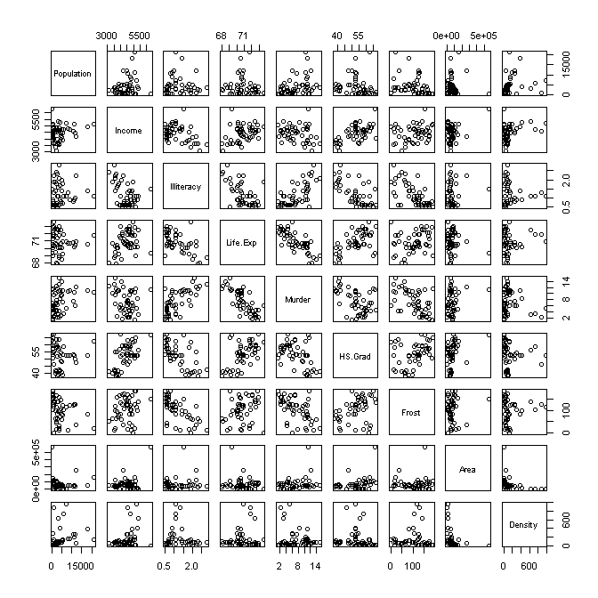
I propose we cast “Life.Exp” into the role of our response variable and attempt to model (predict) it from the other variables. Already we see some interesting relationships. Life expectancy appears to be moderately to strongly related to “Income” (positively), “Illiteracy” (negatively), “Murder” (negatively), HS.Grad (positively), and “Frost” (no. of days per year with frost, positively), and I call particular attention to this last relationship. These are all bivariate relationships–i.e., they don’t take into account any of the remaining variables.
Here’s another interesting relationship, which we would find statistically significant. The correlation between average SAT scores by state and average teacher pay by state is negative. That is to say, the states with higher teacher pay have lower SAT scores. (How much political hay has been made of that? These politicians either don’t understand the nature of regression relationships, or they are spinning the data to tell the story they want you to hear!!) We would also find a very strong negative correlation between SAT scores and percent of eligible students who take the test. I.e., the higher the percentage of HS seniors who take the SAT, the lower the average score. Here is the crucial point. Teacher pay is positively correlated with percent of students who take the test. There is a potential confound here. In regression terms, we would call percent of students who take the test a “lurking variable.”
The advantage of looking at these variables in a multiple regression is we are able to see the relationship between two variables with the others taken out. To say that another way, the regression analysis “holds the potential lurking variables constant” while it is figuring out the relationship between the variables of interest. When SAT scores, teacher pay, and percent taking the test are all entered into the regression relationship, the confound between pay and percent is controlled, and the relationship between teacher pay and SAT scores is shown to be significantly positive.
The point of this long discussion is this. Life expectancy does have a bivariate relationship with a lot of the other variables, but many of those variables are also related to each other. Multiple regression allows us to tease all of this apart and see in a “purer” (but not pure) form what the relationship really is between, say, life expectancy and average number of days with frost. I suggest you watch this relationship as we procede through the analysis.
We should also examine the variables for outliers and distribution before proceding, but for the sake of brevity, we’ll skip it.
The Maximal Model (Sans Interactions)
We begin by throwing all the predictors into a (linear additive) model…
> options(show.signif.stars=F)         # I don't like significance stars!
> names(st)                            # for handy reference
[1] "Population" "Income"     "Illiteracy" "Life.Exp"   "Murder"
[6] "HS.Grad"    "Frost"      "Area"       "Density"
> model1 = lm(Life.Exp ~ Population + Income + Illiteracy + Murder +
+                        HS.Grad + Frost + Area + Density, data=st)
> summary(model1)

Call:
lm(formula = Life.Exp ~ Population + Income + Illiteracy + Murder +
    HS.Grad + Frost + Area + Density, data = st)

Residuals:
     Min       1Q   Median       3Q      Max
-1.47514 -0.45887 -0.06352  0.59362  1.21823

Coefficients:
              Estimate Std. Error t value Pr(>|t|)
(Intercept)  6.995e+01  1.843e+00  37.956  < 2e-16
Population   6.480e-05  3.001e-05   2.159   0.0367
Income       2.701e-04  3.087e-04   0.875   0.3867
Illiteracy   3.029e-01  4.024e-01   0.753   0.4559
Murder      -3.286e-01  4.941e-02  -6.652 5.12e-08
HS.Grad      4.291e-02  2.332e-02   1.840   0.0730
Frost       -4.580e-03  3.189e-03  -1.436   0.1585
Area        -1.558e-06  1.914e-06  -0.814   0.4205
Density     -1.105e-03  7.312e-04  -1.511   0.1385

Residual standard error: 0.7337 on 41 degrees of freedom
Multiple R-squared: 0.7501,     Adjusted R-squared: 0.7013
F-statistic: 15.38 on 8 and 41 DF,  p-value: 3.787e-10
It appears higher populations are related to increased life expectancy and higher murder rates are strongly related to decreased life expectancy. Other than that, we’re not seeing much. Another kind of summary of the model can be obtained like this…
> summary.aov(model1)
            Df  Sum Sq Mean Sq F value    Pr(>F)
Population   1  0.4089  0.4089  0.7597  0.388493
Income       1 11.5946 11.5946 21.5413 3.528e-05
Illiteracy   1 19.4207 19.4207 36.0811 4.232e-07
Murder       1 27.4288 27.4288 50.9591 1.051e-08
HS.Grad      1  4.0989  4.0989  7.6152  0.008612
Frost        1  2.0488  2.0488  3.8063  0.057916
Area         1  0.0011  0.0011  0.0020  0.964381
Density      1  1.2288  1.2288  2.2830  0.138472
Residuals   41 22.0683  0.5383
…but it’s less useful for modeling purposes.
Now we need to start winnowing down our model to a minimal adequate one. The least significant of the slopes in the above summary table was that for “Illiteracy”, but I’ll tell ya what. I kinda want to hold on to “Illiteracy” for awhile, and “Area” was not much better, so I’m going to toss out “Area” first.
The Minimal Adequate Model
We want to reduce our model to a point where all the remaining predictors are significant, and we want to do this by throwing out one predictor at a time. “Area” will go first. To do this, we could just recast the model without the “Area” variable, but R supplies a handier way…
> model2 = update(model1, .~.-Area)
> summary(model2)

Call:
lm(formula = Life.Exp ~ Population + Income + Illiteracy + Murder +
    HS.Grad + Frost + Density, data = st)

Residuals:
    Min      1Q  Median      3Q     Max
-1.5025 -0.4047 -0.0608  0.5868  1.4386

Coefficients:
              Estimate Std. Error t value Pr(>|t|)
(Intercept)  7.094e+01  1.378e+00  51.488  < 2e-16
Population   6.249e-05  2.976e-05   2.100   0.0418
Income       1.485e-04  2.690e-04   0.552   0.5840
Illiteracy   1.452e-01  3.512e-01   0.413   0.6814
Murder      -3.319e-01  4.904e-02  -6.768 3.12e-08
HS.Grad      3.746e-02  2.225e-02   1.684   0.0996
Frost       -5.533e-03  2.955e-03  -1.873   0.0681
Density     -7.995e-04  6.251e-04  -1.279   0.2079

Residual standard error: 0.7307 on 42 degrees of freedom
Multiple R-squared: 0.746,      Adjusted R-squared: 0.7037
F-statistic: 17.63 on 7 and 42 DF,  p-value: 1.173e-10
The syntax of update( ) is cryptic, so here’s what it means. Inside the new formula, a dot means “same.” So read the above update command as follows: “Update model1 using the same response variables and the same predictor variables, except remove (minus) “Area”. Notice that removing “Area” has cost us very little in terms of R-squared, and the adjusted R-squared actually went up, due to there being fewer predictors.
The two models can be compared as follows…
> anova(model1, model2)
Analysis of Variance Table

Model 1: Life.Exp ~ Population + Income + Illiteracy + Murder + HS.Grad +
    Frost + Area + Density
Model 2: Life.Exp ~ Population + Income + Illiteracy + Murder + HS.Grad +
    Frost + Density
  Res.Df     RSS Df Sum of Sq      F Pr(>F)
1     41 22.0683
2     42 22.4247 -1   -0.3564 0.6621 0.4205
As you can see, removing “Area” had no significant effect on the model (p = .4205). Compare the p-value to that for “Area” in the first summary table above. (Ignore the negative sum of squares in this last output. It happened because of the order in which I listed the models. Try it the other way around if you’re unhappy with negative SSs.)
What goes next, “Income” or “Illiteracy”? Fair is fair…
> model3 = update(model2, .~.-Illiteracy)
> summary(model3)

Call:
lm(formula = Life.Exp ~ Population + Income + Murder + HS.Grad +
    Frost + Density, data = st)

Residuals:
     Min       1Q   Median       3Q      Max
-1.49555 -0.41246 -0.05336  0.58399  1.50535

Coefficients:
              Estimate Std. Error t value Pr(>|t|)
(Intercept)  7.131e+01  1.042e+00  68.420  < 2e-16
Population   5.811e-05  2.753e-05   2.110   0.0407
Income       1.324e-04  2.636e-04   0.502   0.6181
Murder      -3.208e-01  4.054e-02  -7.912 6.32e-10
HS.Grad      3.499e-02  2.122e-02   1.649   0.1065
Frost       -6.191e-03  2.465e-03  -2.512   0.0158
Density     -7.324e-04  5.978e-04  -1.225   0.2272

Residual standard error: 0.7236 on 43 degrees of freedom
Multiple R-squared: 0.745,      Adjusted R-squared: 0.7094
F-statistic: 20.94 on 6 and 43 DF,  p-value: 2.632e-11
Things are starting to change a bit. R-squared went down again, as it will always do when a predictor is removed, but once more adjusted R-squared increased. “Frost” is also now a significant predictor of life expectancy, and unlike in the bivariate relationship we saw originally, the relationship is now negative.
Looks like income should go next…
> model4 = update(model3, .~.-Income)
> summary(model4)

Call:
lm(formula = Life.Exp ~ Population + Murder + HS.Grad + Frost +
    Density, data = st)

Residuals:
     Min       1Q   Median       3Q      Max
-1.56877 -0.40951 -0.04554  0.57362  1.54752

Coefficients:
              Estimate Std. Error t value Pr(>|t|)
(Intercept)  7.142e+01  1.011e+00  70.665  < 2e-16
Population   6.083e-05  2.676e-05   2.273  0.02796
Murder      -3.160e-01  3.910e-02  -8.083 3.07e-10
HS.Grad      4.233e-02  1.525e-02   2.776  0.00805
Frost       -5.999e-03  2.414e-03  -2.485  0.01682
Density     -5.864e-04  5.178e-04  -1.132  0.26360

Residual standard error: 0.7174 on 44 degrees of freedom
Multiple R-squared: 0.7435,     Adjusted R-squared: 0.7144
F-statistic: 25.51 on 5 and 44 DF,  p-value: 5.524e-12
R-squared went down hardly at all. Adjusted R-squared went up. “Illiteracy” will not be missed.
Now all the predictors are significant except “Density”…
> model5 = update(model4, .~.-Density)
> summary(model5)

Call:
lm(formula = Life.Exp ~ Population + Murder + HS.Grad + Frost,
    data = st)

Residuals:
     Min       1Q   Median       3Q      Max
-1.47095 -0.53464 -0.03701  0.57621  1.50683

Coefficients:
              Estimate Std. Error t value Pr(>|t|)
(Intercept)  7.103e+01  9.529e-01  74.542  < 2e-16
Population   5.014e-05  2.512e-05   1.996  0.05201
Murder      -3.001e-01  3.661e-02  -8.199 1.77e-10
HS.Grad      4.658e-02  1.483e-02   3.142  0.00297
Frost       -5.943e-03  2.421e-03  -2.455  0.01802

Residual standard error: 0.7197 on 45 degrees of freedom
Multiple R-squared: 0.736,      Adjusted R-squared: 0.7126
F-statistic: 31.37 on 4 and 45 DF,  p-value: 1.696e-12
Adjusted R-squared slipped a bit that time, but not significantly as we could confirm by…
> anova(model5, model4) # output not shown
We have (implicitly by not saying otherwise) set our alpha level at .05, so now “Population” must go. This could have a substantial effect on the model, as the slope for “Population” is very nearly significant. Only one way to find out…
> model6 = update(model5, .~.-Population)
> summary(model6)

Call:
lm(formula = Life.Exp ~ Murder + HS.Grad + Frost, data = st)

Residuals:
    Min      1Q  Median      3Q     Max
-1.5015 -0.5391  0.1014  0.5921  1.2268

Coefficients:
             Estimate Std. Error t value Pr(>|t|)
(Intercept) 71.036379   0.983262  72.246  < 2e-16
Murder      -0.283065   0.036731  -7.706 8.04e-10
HS.Grad      0.049949   0.015201   3.286  0.00195
Frost       -0.006912   0.002447  -2.824  0.00699

Residual standard error: 0.7427 on 46 degrees of freedom
Multiple R-squared: 0.7127,     Adjusted R-squared: 0.6939
F-statistic: 38.03 on 3 and 46 DF,  p-value: 1.634e-12
We have reached the minimal adequate model.
Stepwise Regression
What we did in the previous section can be automated using the step( ) function…
> step(model1, direction="backward")
Start:  AIC=-22.89
Life.Exp ~ Population + Income + Illiteracy + Murder + HS.Grad +
    Frost + Area + Density

             Df Sum of Sq     RSS     AIC
- Illiteracy  1     0.305  22.373 -24.208
- Area        1     0.356  22.425 -24.093
- Income      1     0.412  22.480 -23.969
                     22.068 -22.894
- Frost       1     1.110  23.178 -22.440
- Density     1     1.229  23.297 -22.185
- HS.Grad     1     1.823  23.891 -20.926
- Population  1     2.510  24.578 -19.509
- Murder      1    23.817  45.886  11.706

Step:  AIC=-24.21
Life.Exp ~ Population + Income + Murder + HS.Grad + Frost + Area +
    Density

             Df Sum of Sq     RSS     AIC
- Area        1     0.143  22.516 -25.890
- Income      1     0.232  22.605 -25.693
                     22.373 -24.208
- Density     1     0.929  23.302 -24.174
- HS.Grad     1     1.522  23.895 -22.917
- Population  1     2.205  24.578 -21.508
- Frost       1     3.132  25.506 -19.656
- Murder      1    26.707  49.080  13.072

Step:  AIC=-25.89
Life.Exp ~ Population + Income + Murder + HS.Grad + Frost + Density

             Df Sum of Sq     RSS     AIC
- Income      1     0.132  22.648 -27.598
- Density     1     0.786  23.302 -26.174
                     22.516 -25.890
- HS.Grad     1     1.424  23.940 -24.824
- Population  1     2.332  24.848 -22.962
- Frost       1     3.304  25.820 -21.043
- Murder      1    32.779  55.295  17.033

Step:  AIC=-27.6
Life.Exp ~ Population + Murder + HS.Grad + Frost + Density

             Df Sum of Sq     RSS     AIC
- Density     1     0.660  23.308 -28.161
                     22.648 -27.598
- Population  1     2.659  25.307 -24.046
- Frost       1     3.179  25.827 -23.030
- HS.Grad     1     3.966  26.614 -21.529
- Murder      1    33.626  56.274  15.910

Step:  AIC=-28.16
Life.Exp ~ Population + Murder + HS.Grad + Frost

             Df Sum of Sq     RSS     AIC
                     23.308 -28.161
- Population  1     2.064  25.372 -25.920
- Frost       1     3.122  26.430 -23.876
- HS.Grad     1     5.112  28.420 -20.246
- Murder      1    34.816  58.124  15.528

Call:
lm(formula = Life.Exp ~ Population + Murder + HS.Grad + Frost,     data = st)

Coefficients:
(Intercept)   Population       Murder      HS.Grad        Frost
  7.103e+01    5.014e-05   -3.001e-01    4.658e-02   -5.943e-03
…but I’m against it! The “direction=” option can be set to “forward”, “backward”, or “both”.
Confidence Limits on the Estimated Coefficients
Easy…
> confint(model6)
                  2.5 %       97.5 %
(Intercept) 69.05717472 73.015582905
Murder      -0.35700149 -0.209128849
HS.Grad      0.01935043  0.080546980
Frost       -0.01183825 -0.001985219
Set the desired confidence level with the “level=” option (not conf.level as in many other R functions).
Predictions
Predictions can be made from a model equation using the predict( ) function…
> predict(model6, list(Murder=10.5, HS.Grad=48, Frost=100))
       1
69.77056
Feed it the model name and a list of labeled values for the predictors. The values to be predicted from can be vectors.
Regression Diagnostics
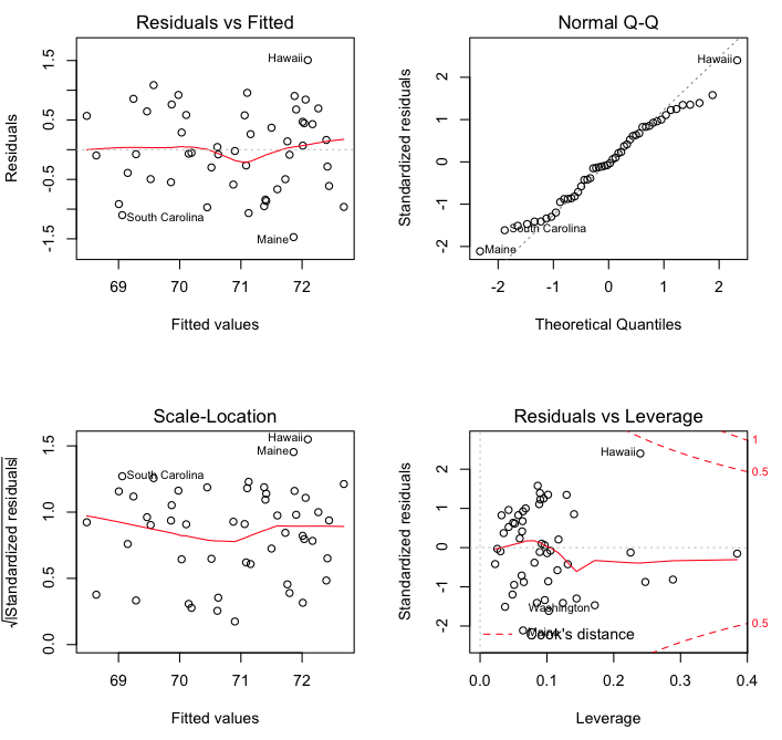
The usual diagnostic plots are available…
> par(mfrow=c(2,2))                    # visualize four graphs at once
> plot(model6)
> par(mfrow=c(1,1))                    # reset the graphics defaults
Extracting Elements of the Model Object
The model data object is a list containing quite a lot of information. Aside from the summary functions we used above, there are two ways to get at this information…
> model6[[1]]                          # extract list item 1: coefficients
 (Intercept)       Murder      HS.Grad        Frost
71.036378813 -0.283065168  0.049948704 -0.006911735
> model6[[2]]                          # extract list item 2: residuals
       Alabama         Alaska        Arizona       Arkansas     California
    0.36325842    -0.80873734    -1.07681421     0.93888883     0.60063821
      Colorado    Connecticut       Delaware        Florida        Georgia
    0.90409006     0.48472687    -1.23666537     0.10114571    -0.17498630
        Hawaii          Idaho       Illinois        Indiana           Iowa
    1.22680042     0.23279723     0.26968086     0.05432904     0.19534036
        Kansas       Kentucky      Louisiana          Maine       Maryland
    0.61342480     0.79770164    -0.56481311    -1.50150772    -0.32455693
 Massachusetts       Michigan      Minnesota    Mississippi       Missouri
   -0.48235430     0.96231978     0.80350324    -1.11037437     0.59509781
       Montana       Nebraska         Nevada  New Hampshire     New Jersey
   -0.94669741     0.38328311    -0.70837880    -0.54666731    -0.46189744
    New Mexico       New York North Carolina   North Dakota           Ohio
    0.10159299     0.53349703    -0.05444180     0.91307523     0.07808745
      Oklahoma         Oregon   Pennsylvania   Rhode Island South Carolina
    0.18464735    -0.41031105    -0.51622769     0.10314800    -1.23162114
  South Dakota      Tennessee          Texas           Utah        Vermont
    0.05138438     0.58330361     1.19135836     0.72277428     0.46958000
      Virginia     Washington  West Virginia      Wisconsin        Wyoming
   -0.06731035    -1.04976581    -1.04653483     0.60046076    -0.73927257
There are twelve elements in this list. They can also be extracted by name, and the supplied name only has to be long enough to be recognized. So instead of asking for list item 2, you can ask for…
> sort(model6$resid)                   # extract residuals and sort them
         Maine       Delaware South Carolina    Mississippi        Arizona
   -1.50150772    -1.23666537    -1.23162114    -1.11037437    -1.07681421
    Washington  West Virginia        Montana         Alaska        Wyoming
   -1.04976581    -1.04653483    -0.94669741    -0.80873734    -0.73927257
        Nevada      Louisiana  New Hampshire   Pennsylvania  Massachusetts
   -0.70837880    -0.56481311    -0.54666731    -0.51622769    -0.48235430
    New Jersey         Oregon       Maryland        Georgia       Virginia
   -0.46189744    -0.41031105    -0.32455693    -0.17498630    -0.06731035
North Carolina   South Dakota        Indiana           Ohio        Florida
   -0.05444180     0.05138438     0.05432904     0.07808745     0.10114571
    New Mexico   Rhode Island       Oklahoma           Iowa          Idaho
    0.10159299     0.10314800     0.18464735     0.19534036     0.23279723
      Illinois        Alabama       Nebraska        Vermont    Connecticut
    0.26968086     0.36325842     0.38328311     0.46958000     0.48472687
      New York      Tennessee       Missouri      Wisconsin     California
    0.53349703     0.58330361     0.59509781     0.60046076     0.60063821
        Kansas           Utah       Kentucky      Minnesota       Colorado
    0.61342480     0.72277428     0.79770164     0.80350324     0.90409006
  North Dakota       Arkansas       Michigan          Texas         Hawaii
    0.91307523     0.93888883     0.96231978     1.19135836     1.22680042
That settles it! I’m moving to Hawaii. (This could all just be random error, of course, but more technically, it is unexplained variation. It could mean that Maine is performing the worst against our model, and Hawaii the best, due to factors we have not included in the model.)
Beta Coeffieicents
Beta or standardized coefficients are the slopes we would get if all the variables were on the same scale, which is done by converting them to z-scores before doing the regression. Betas allow a comparison of the relative importance of the predictors, which neither the unstandardized coefficients nor the p-values does. Scaling, or standardizing, the data vectors can be done using the scale( ) function…
> model7 = lm(scale(Life.Exp) ~ scale(Murder) + scale(HS.Grad) + scale(Frost),
+                               data=st)
> summary(model7)

Call:
lm(formula = scale(Life.Exp) ~ scale(Murder) + scale(HS.Grad) +
    scale(Frost), data = st)

Residuals:
     Min       1Q   Median       3Q      Max
-1.11853 -0.40156  0.07551  0.44111  0.91389

Coefficients:
                 Estimate Std. Error  t value Pr(>|t|)
(Intercept)    -4.541e-15  7.824e-02 -5.8e-14  1.00000
scale(Murder)  -7.784e-01  1.010e-01   -7.706 8.04e-10
scale(HS.Grad)  3.005e-01  9.146e-02    3.286  0.00195
scale(Frost)   -2.676e-01  9.477e-02   -2.824  0.00699

Residual standard error: 0.5532 on 46 degrees of freedom
Multiple R-squared: 0.7127,     Adjusted R-squared: 0.6939
F-statistic: 38.03 on 3 and 46 DF,  p-value: 1.634e-12
The intercept goes to zero, and the slopes become standardized beta values. So an increase of one standard deviation in the murder rate is associated with a drop of 0.778 standard deviations in life expectancy, if all the other variables are held constant. VERY roughly, these values can be interpreted as correlations with the other predictors controlled. The same result could have been obtained via the formula for standardized coefficients…
> -0.283 * sd(st$Murder) / sd(st$Life.Exp)
[1] -0.778241
Where the first value is the unstandardized coefficient for “Murder”.
Partial Correlations
Another way to remove the effect of a possible lurking variable from the correlation of two other variables is to calculate a partial correlation. There is no partial correlation function in R. So to create one, copy and paste this script into the R Console…
### Partial correlation coefficient
### From formulas in Sheskin, 3e
### a,b=variables to be correlated, c=variable to be partialled out of both
pcor = function(a,b,c)
{
     (cor(a,b)-cor(a,c)*cor(b,c))/sqrt((1-cor(a,c)^2)*(1-cor(b,c)^2))
}
### end of script
This will put a function called pcor( ) in your workspace. To use it, enter the names of the variables you want the partial correlation of first, and then enter the name of the variable you want partialled out (controlled)…
> pcor(st$Life.Exp, st$Murder, st$HS.Grad)
[1] -0.6999659
The partial correlation between “Life.Exp” and “Murder” with “HS.Grad” held constant is about -0.7.
Making Predictions From a Model
To illustrate how predictions are made from a model, I will fit a new model to another data set…
> rm(list=ls())                        # clean up (WARNING! this will wipe your workspace!)
> data(airquality)                     # see ?airquality for details on these data
> na.omit(airquality) -> airquality    # toss cases with missing values
> lm(Ozone ~ Solar.R + Wind + Temp + Month,
             data=airquality) -> model
> coef(model)
 (Intercept)      Solar.R         Wind         Temp        Month
-58.05383883   0.04959683  -3.31650940   1.87087379  -2.99162786
The model has been fitted and the regression coefficients displayed. Suppose now we wish to predict for new values: Solar.R=200, Wind=11, Temp=80, Month=6. One way to do it is this…
> (prediction <- c(1,200,11,80,6) * coef(model))
(Intercept)     Solar.R        Wind        Temp       Month
 -58.053839    9.919365  -36.481603  149.669903  -17.949767
> ### Note: putting the whole statement in parentheses not only stores the values
> ###       but also prints them to the Console.
> sum(prediction)
[1] 47.10406
Our predicted value is 47.1. How accurate is it?
We can get a confidence interval for the predicted value, but first we have to ask an important question. Is the prediction being made for the mean response for cases like this? Or is it being made for a new single case? The difference this makes to the CI is shown below…
### Prediction of mean response for cases like this...
> predict(model, list(Solar.R=200,Wind=11,Temp=80,Month=6), interval="conf")
       fit      lwr      upr
1 47.10406 41.10419 53.10393
### Prediction for a single new case...
> predict(model, list(Solar.R=200,Wind=11,Temp=80,Month=6), interval="pred")
       fit      lwr      upr
1 47.10406 5.235759 88.97236
As you can see, the CI is much wider in the second case. These are 95% CIs. You can set a different confidence level using the “level=” option. The function predict( ) has a somewhat tricky syntax, so here’s how it works. The first argument should be the name of the model object. The second argument should be a list of new data values labeled with the variables names. That’s all that’s really required. The “interval=” option can take values of “none” (the default), “confidence”, or “prediction”. You need only type enough of it so R knows which one you want. The confidence level is changed with the “level=” option, and not with “conf.level=” as in other R functions.