Anyone familiar with transportation modeling is familiar with processes that iterate through data. Gravity models iterate, feedback loops iterate, assignment processes iterate (well, normally), model estimation processes iterate, gravity model calibration steps, shadow cost loops iterate… the list goes on.
Sometimes it’s good to see what is going on during those iterations, especially with calibration. For example, in calibrating friction factors in a gravity model, I’ve frequently run around 10 iterations. However, as an experiment I set the iterations on a step to 100 and looked at the result:
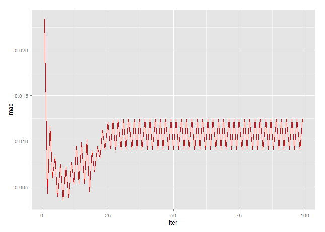
This is the mean absolute error in percentage of observed trips to modeled trips in distribution. Note the oscillation that starts around iteration 25 – this was not useful nor detected. Note also that the best point was very early in the iteration process – at iteration 8.
After telling these files to save after each iteration (an easy process), I faced the issue of trying to quickly read 99 files and get some summary statistics. Writing that in R was not only the path of least resistance, it was so fast to run that it was probably the fastest solution. The code I used is below, with comments:
|
library(foreign)
library(ggplot2)
#This is where my files are at
setwd(“C:\\Modelrun\\10a10b10a08aV80”)
#This is the data frame that will hold the output statistics
stats<-data.frame(iter=1:99,mae=0,mse=0)
#Loop through files
#
# The files are named 4dNHBPKTLFComp_ITnn.DBF, where nn goes from 01-99
for(i in 1:99){
#Build the filename
if(i<10){
fname=paste(“4dNHBPKTLFComp_It0″,i,”.dbf”,sep=””)
}else{
fname=paste(“4dNHBPKTLFComp_It”,i,”.dbf”,sep=””)
}
#Open the file
intab<-read.dbf(fname)
#Run the stats – mean absolute error (MAE) and mean square error (MSE)
stats[i,2]=mean(abs(intab$OBSTLF-intab$MODELTLF))
stats[i,3]=mean((intab$OBSTLF-intab$MODELTLF)^2)
}
#Plot the results
maeplot<-ggplot(data=stats,aes(x=iter,y=mae))+geom_line(color=’red’,size=0.5)
mseplot<-ggplot(data=stats,aes(x=iter,y=mse))+geom_line(color=’red’,size=0.5)
|