Collinearity, or excessive correlation among explanatory variables, can complicate or prevent the identification of an optimal set of explanatory variables for a statistical model. For example, forward or backward selection of variables could produce inconsistent results, variance partitioning analyses may be unable to identify unique sources of variation, or parameter estimates may include substantial amounts of uncertainty. The temptation to build an ecological model using all available information (i.e., all variables) is hard to resist. Lots of time and money are exhausted gathering data and supporting information. We also hope to identify every significant variable to more accurately characterize relationships with biological relevance. Analytical limitations related to collinearity require us to think carefully about the variables we choose to model, rather than adopting a naive approach where we blindly use all information to understand complexity. The purpose of this blog is to illustrate use of some techniques to reduce collinearity among explanatory variables using a simulated dataset with a known correlation structure.
A simple approach to identify collinearity among explanatory variables is the use of variance inflation factors (VIF). VIF calculations are straightforward and easily comprehensible; the higher the value, the higher the collinearity. A VIF for a single explanatory variable is obtained using the r-squared value of the regression of that variable against all other explanatory variables:

where the 


Several packages in R provide functions to calculate VIF: vif in package HH, vifin package car, VIF in package fmsb, vif in package faraway, and vif in package VIF. The number of packages that provide VIF functions is surprising given that they all seem to accomplish the same thing. One exception is the function in the VIF package, which can be used to create linear models using VIF-regression. The nuts and bolts of this function are a little unclear since the documentation for the package is sparse. However, what this function does accomplish is something that the others do not: stepwise selection of variables using VIF. Removing individual variables with high VIF values is insufficient in the initial comparison using the full set of explanatory variables. The VIF values will change after each variable is removed. Accordingly, a more thorough implementation of the VIF function is to use a stepwise approach until all VIF values are below a desired threshold. For example, using the full set of explanatory variables, calculate a VIF for each variable, remove the variable with the single highest value, recalculate all VIF values with the new set of variables, remove the variable with the next highest value, and so on, until all values are below the threshold.
In this blog we’ll use a custom function for stepwise variable selection. I’ve created this function because I think it provides a useful example for exploring stepwise VIF analysis. The function is a wrapper for the vif function in fmsb. We’ll start by simulating a dataset with a known correlation structure.
require(MASS)
require(clusterGeneration)

set.seed(2)
num.vars<-15
num.obs<-200
cov.mat<-genPositiveDefMat(num.vars,covMethod="unifcorrmat")$Sigma
rand.vars<-mvrnorm(num.obs,rep(0,num.vars),Sigma=cov.mat)
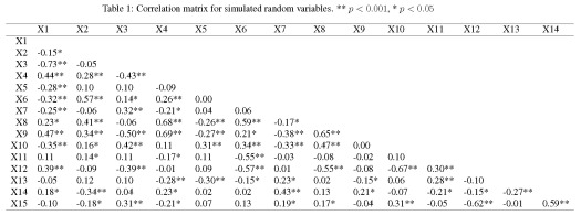
We’ve created fifteen ‘explanatory’ variables with 200 observations each. Themvrnorm function (MASS package) was used to create the data using a covariance matrix from the genPositiveDefMat function (clusterGeneration package). These functions provide a really simple approach to creating data matrices with arbitrary correlation structures. The covariance matrix was chosen from a uniform distribution such that some variables are correlated while some are not. A more thorough explanation about creating correlated data matrices can be found here. The correlation matrix for the random variables should look very similar to the correlation matrix from the actual values (as sample size increases, the correlation matrix approaches cov.mat).
Now we create our response variable as a linear combination of the explanatory variables. First, we create a vector for the parameters describing the relationship of the response variable with the explanatory variables. Then, we use some matrix algebra and a randomly distributed error term to create the response variable. This is the standard form for a linear regression model.
parms<-runif(num.vars,-10,10)
y<-rand.vars %*% matrix(parms) + rnorm(num.obs,sd=20)
We would expect a regression model to indicate each of the fifteen explanatory variables are significantly related to the response variable, since we know the true relationship of y with each of the variables. However, our explanatory variables are correlated. What happens when we create the model?
lm.dat<-data.frame(y,rand.vars)
form.in<-paste('y ~',paste(names(lm.dat)[-1],collapse='+'))
mod1<-lm(form.in,data=lm.dat)
summary(mod1)
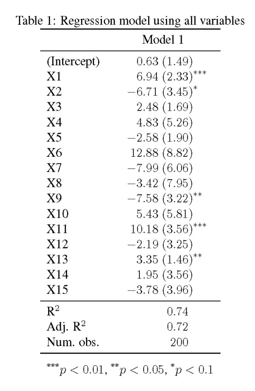
The model shows that only four of the fifteen explanatory variables are significantly related to the response variable (at 
We can try an alternative approach to building the model that accounts for collinearity among the explanatory variables. We can implement the custom VIF function as follows.
vif_func(in_frame=rand.vars,thresh=5,trace=T)

  var vif
 X1  26.7776302460193
 X2  35.7654696801389
 X3  14.8902623488606
 X4  50.6259723278776
 X5  10.599371257556
 X6  108.343545737888
 X7  48.2508656429107
 X8  183.136179797657
 X9  51.6790552123906
 X10 63.8699838164383
 X11 38.9458133633031
 X12 44.3534264537944
 X13 9.35861427426385
 X14 63.1574276237521
 X15 30.0137537949494

removed:  X8 183.1362

 var vif
 X1  5.57731851381497
 X2  10.0195886727232
 X3  5.55663566788945
 X4  6.8064112804091
 X5  9.7815324084451
 X6  22.3236741700758
 X7  36.854990561001
 X9  16.972399679086
 X10 57.2665930293009
 X11 22.4854807367867
 X12 43.1006397357538
 X13 8.54661668063361
 X14 29.7536838039265
 X15 21.6340334562738

removed:  X10 57.26659

 var vif
 X1  5.55463656650283
 X2  8.43692519123461
 X3  4.20157496220101
 X4  4.30562228649632
 X5  1.85152657224351
 X6  9.78518916197122
 X7  3.59917695249808
 X9  5.62398393809027
 X11 4.32732961231283
 X12 8.92901049257853
 X13 2.22079922858869
 X14 9.73258301210856
 X15 8.69287102590565

removed:  X6 9.785189

 var vif
 X1  4.88431271981048
 X2  3.0066710371039
 X3  3.92223104412672
 X4  4.03552281755132
 X5  1.85130973105683
 X7  3.56687077767566
 X9  5.55536287729148
 X11 2.11226533056043
 X12 5.58689916270725
 X13 1.86868960383407
 X14 9.39686287473867
 X15 7.80042398111767

removed:  X14 9.396863

[1] "X1"  "X2"  "X3"  "X4"  "X5"  "X7"  "X9"  "X11"
 [9] "X12" "X13" "X15"
The function uses three arguments. The first is a matrix or data frame of the explanatory variables, the second is the threshold value to use for retaining variables, and the third is a logical argument indicating if text output is returned as the stepwise selection progresses. The output indicates the VIF values for each variable after each stepwise comparison. The function calculates the VIF values for all explanatory variables, removes the variable with the highest value, and repeats until all VIF values are below the threshold. The final output is a list of variable names with VIF values that fall below the threshold. Now we can create a linear model using explanatory variables with less collinearity.
keep.dat<-vif_func(in_frame=rand.vars,thresh=5,trace=F)
form.in<-paste('y ~',paste(keep.dat,collapse='+'))
mod2<-lm(form.in,data=lm.dat)
summary(mod2)
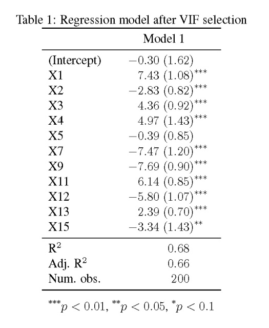
The updated regression model is much improved over the original. We see an increase in the number of variables that are significantly related to the response variable. This increase is directly related to the standard error estimates for the parameters, which look at least 50% smaller than those in the first model. The take home message is that true relationships among variables will be masked if explanatory variables are collinear. This creates problems in model creation which lead to complications in model inference. Taking the extra time to evaluate collinearity is a critical first step to creating more robust ecological models.
Function and example code:
#stepwise VIF function used below
vif_func<-function(in_frame,thresh=10,trace=T,...){

  require(fmsb)

  if(class(in_frame) != 'data.frame') in_frame<-data.frame(in_frame)

  #get initial vif value for all comparisons of variables
  vif_init<-NULL
  for(val in names(in_frame)){
      form_in<-formula(paste(val,' ~ .'))
      vif_init<-rbind(vif_init,c(val,VIF(lm(form_in,data=in_frame,...))))
      }
  vif_max<-max(as.numeric(vif_init[,2]))

  if(vif_max < thresh){
    if(trace==T){ #print output of each iteration
        prmatrix(vif_init,collab=c('var','vif'),rowlab=rep('',nrow(vif_init)),quote=F)
        cat('\n')
        cat(paste('All variables have VIF < ', thresh,', max VIF ',round(vif_max,2), sep=''),'\n\n')
        }
    return(names(in_frame))
    }
  else{

    in_dat<-in_frame

    #backwards selection of explanatory variables, stops when all VIF values are below 'thresh'
    while(vif_max >= thresh){

      vif_vals<-NULL

      for(val in names(in_dat)){
        form_in<-formula(paste(val,' ~ .'))
        vif_add<-VIF(lm(form_in,data=in_dat,...))
        vif_vals<-rbind(vif_vals,c(val,vif_add))
        }
      max_row<-which(vif_vals[,2] == max(as.numeric(vif_vals[,2])))[1]

      vif_max<-as.numeric(vif_vals[max_row,2])

      if(vif_max<thresh) break

      if(trace==T){ #print output of each iteration
        prmatrix(vif_vals,collab=c('var','vif'),rowlab=rep('',nrow(vif_vals)),quote=F)
        cat('\n')
        cat('removed: ',vif_vals[max_row,1],vif_max,'\n\n')
        flush.console()
        }

      in_dat<-in_dat[,!names(in_dat) %in% vif_vals[max_row,1]]

      }

    return(names(in_dat))

    }

  }