Prerequisite: Planning 2 or dean's permission
Units: 3.0
Classroom: online via Microsoft Teams
Class Time: Thursday: 9:30 AM-12:30 PM
Office Hour: Thursday: 12:30 PM -12:45 PM - Right after class time
Instructor: Zhuo Yao, Ph.D.
Instructor: Archt. Carmela C. Quizana
Travel simulations require that an urban area be represented as a series of small geographic areas called travel analysis zones (TAZs). Zones are characterized by their population, employment and other factors and are the places where trip making decisions are made (trip producers) and the trip need is met (trip attractors). Trip making is assumed to begin at the center of activity in a zone (zone centroid). Trips that are very short, that begin and end in a single zone (intrazonal trips) are usually not directly included in the forecasts. This limits the analysis of pedestrian and bicycle trips in the process. Zones can be as small as a single block but typically are 1/4 to one mile square in area. A planning study can easily use 500-2000 zones. A large number of zones will increase the accuracy of the forecasts but require more data and computer processing time. Zones tend to be small in areas of high population and larger in more rural areas. Internal zones are those within the study area while external zones are those outside of the study area. The study area should be large enough so that nearly all (over 90%) of the trips begin and end within the study area.
The highway system and transit systems are represented as networks for computer analysis. Networks consist of links to represent segments of highways or transit lines and nodes to represent intersections and other points on the network. Data for links includes travel times on the link, average speeds, capacity, and direction. Node data is more limited to information on which links connect to the node and the location of the node (coordinates). Node data could also include data on intersections to help calculate delay encountered at intersections.
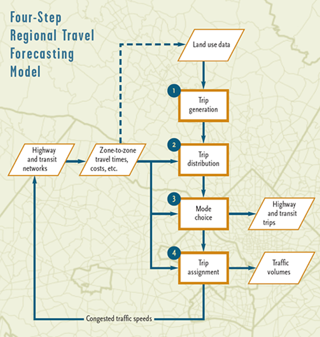
The travel simulation process follows trips as they begin at a trip generation zone, move through a network of links and nodes and end at a trip attracting zone. The simulation process is known as the four step process for the steps of trip generation, trip distribution, mode split and traffic assignment.
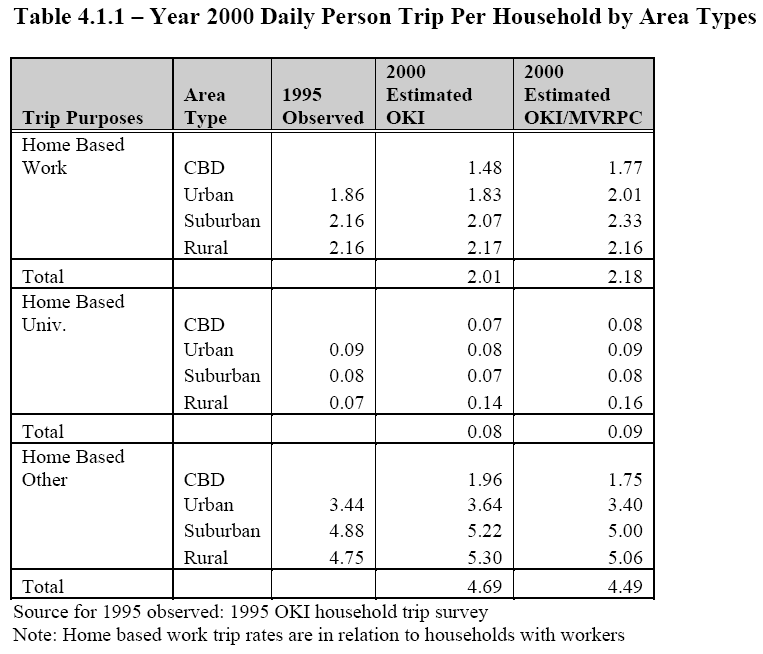
The first step in travel forecasting is trip generation. In this step information from land use, population and economic forecasts are used to estimate how many trips will be made to and from each zone.
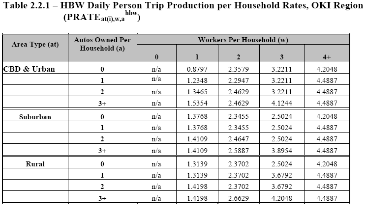
This is done separately by trip purpose. Some of the trip purposes that could be used are: home based work trips (work trips that begin or end at home), home based shopping trips, home based other trips, school trips, non-home based trips (trips that neither begin or end at home), truck trips and taxi trips. Trips are calculated based on the characteristics of the zones. Trip productions are based on household characteristics such as the number of people in the household and the number of vehicles available. For example a household with four people and two vehicles may be assumed to produce 3.00 work trips per day. Trip attractions are typically based on the level of employment in a zone. For example a zone could be assumed to attract 1.32 home based work trips for every person employed in that zone. Trip generation uses trip rates that are averages for large segments of the study area.
Assumptions and limitations: Some of the assumptions in trip generation are as follows:
Independent decisions. Travel behavior is a complex process where often decisions of one household member are dependent on others in the household. For example, child care needs may affect how and when people travel to other places. This interdependency for trip making is not considered.
Limited trip purposes. With no more than four to eight trip purposes, a simplified trip pattern results. All shopping trips are treated the same weather shopping for groceries or lumber. Home based "other" trip purposes cover a wide variety of purposes - medical, visit friends, banking, etc. which are influenced by a wider variety of factors than those used in the modeling process.
Combinations of trips are ignored. Travelers may often combine a variety of purposes into a sequence of trips as the run errands and link together activities. This is called trip chaining and is a complex process. The modeling process treats such trip combinations in a very limited way.
Feedback, cause and effect problems. Trip generation models sometimes calculate trips as a function of factors that in turn could depend on how many trips there are. For example shopping trip attractions are found as a function of retail employment, but it could also be argued that the number of retail employees at a shopping center will depend on how many people come there to shop. This 'chicken and egg' problem comes up frequently in travel forecasts and is difficult to avoid. Another example is that trip making depends on auto availability, but it could be also argued that the number of automobiles a household owns would depend upon how active they are in making trips.
Trip generation only finds the number of trips that begin or end at a particular zone.
The process of trip distribution links the trip ends to form an origin-destination pattern.
Trip distribution is used to represent the process of destination choice, i.e. "I need to go shopping but where should I go to meet my shopping needs?. Trip distribution leads to a large increase in the amount of data which needs to be dealt with. Origin-destination tables are very large. For example a 1200 zone study area would have 1,440,000 possible trip combinations in its O-D table for each trip purpose. The most commonly used procedure for trip distribution is called the gravity model. The gravity model takes the trips produced at one zone and distributes to other zones based on the size of the other zones (as measured by their trip attractions) and on the basis of the distance to other zones. A zone with a large number of trip attractions (say a large shopping center) will receive a greater number of distributed trips than one with a small trip attractions ( a small shopping center). Distance to possible destinations is the other factor used in the gravity model. The number of trips to a given destination decreases with the distance to the destination (it is inversely proportional). For example, you would expect more trips to a nearby shopping center than one further away. The distance effect is found through a calibration process which gives travel times to destinations from the model similar to that found from field data. "Distance” can be measured several ways. The simplest way this is done is to use auto travel times between zones is as the measurement of distance. Other ways might be to use a combination of auto travel time and costs such as tolls as the measurement of distance. Still another way is to use a combination of transit and auto times and costs (composite cost). This method involves using a percentage of the auto time and cost and a percentage of the transit time/cost. Because of calculation procedures, the model must be used a number of times (iterated) in order to balance the trip numbers to match the initial values.
Assumptions and limitations: Some of the assumptions in trip distribution are as follows:
Constant trip times: In order for the model to be used as a forecasting tool it must be assumed that the average lengths of trips that occur now will remain constant in the future. Since trip lengths are measured by travel time this means that improvements in the transportation system that reduce travel times are assumed to be balanced by a further separation of origins and destinations. Thus faster speeds on the network will result in longer trips, measured by distance.
Use of automobile travel times to represent 'distance'. The gravity model requires a measurement of the distance between zones. This is almost always based on automobile travel times rather than transit travel times and leads to a wider distribution of trips (they are spread out over a wider radius of places) than if transit times were used. This process limits the ability to represent travel patterns of households that locate on a transit route and travel to points along that route.
Limited effect of social-economic-cultural factors. The gravity model distributes trips only on the basis of size of the trip ends (trip productions, trip attractions) and travel times between the trip ends. Thus the model would predict a large number of trips between a high income residential area and a nearby low income employment area or between a Spanish speaking neighborhood and a nearly non-Spanish speaking neighborhood. The actual distribution of trips is affected by the nature of the people and activities that are involved and their socio-economic and cultural characteristics as well as the size and distance factors used in the model. Furthermore, groups of travelers might avoid some areas of the city and favor others based on socio-economic-cultural reasons. Adjustments are sometimes made in the model to account for such factors, but it is difficult since the effects of these factors on travel is difficult to quantify much less to predict how it would change over time.
Feedback problems: Travel times are needed to calculate trip distribution; however travel times depend upon the level of congestion on streets in the network. The level of congestion is not known during the trip distribution step since that is found in a later calculation. Normally what is done is that travel times are assumed and checked later. If the assumed values differ from the actual values, they should be modified and the calculations should be redone.
Mode choice is one of the most critical parts of the demand modeling process.
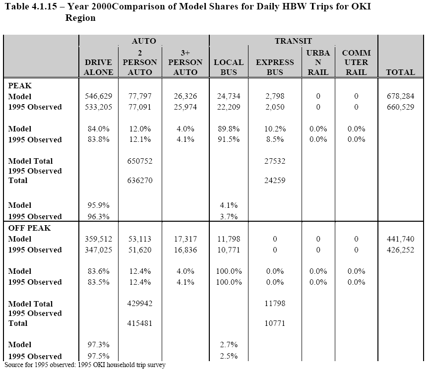
It is the step where trips between a given origin and destination are split into trips using transit, trips by car pool or as automobile passengers and trips by automobile drivers.
Calculations are conducted that compare the attractiveness of travel by different modes to determine their relative usage. All proposals to improve public transit or to change the ease of using the automobile are passed through the mode split/auto occupancy process as part of their assessment and evaluation. It is important to understand what factors are used and how the process is conducted in order to plan, design and implement new systems of transportation.
Mode split is done by a comparison of the "disutility" of travel between two points for the different modes that are available. Disutility is a term used to represent a combination of the travel time, cost and convenience of a mode between an origin and a destination. It is found by placing multipliers (weights) on these factors and adding them together. Travel time is divided into two components: in-vehicle time to represent the time when a traveler is actually in a vehicle and moving and out-of-vehicle time which includes time spend traveling which occurs outside of the vehicle (time to walk to and from transit stops, waiting time, transfer time). Out-of-vehicle time is used to represent "convenience" and is typically multiplied by a factor of 2.0 to 7.0 to give it greater importance in the calculations. This is because travelers do not like to wait or walk long distances to their destinations. The size of the multiplier will be different depending upon the purpose of the trip. Travel cost is multiplied by a factor to represent the value that travelers place on time savings for a particular trip purpose. For transit trips, the cost of the trip is given as the average transit fare for that trip while for auto trips cost is found by adding the parking cost to the length of the trip as multiplied by a cost per mile. Auto cost is based on a "perceived" cost per mile (on the order of 5-10 cents/mile) which only includes fuel and oil costs and does not include ownership, insurance, maintenance and other fixed costs (total costs of automobile travel are much higher). Disutility calculations may also contain a "mode bias factor" which is used to represent other characteristics or travel modes which may influence the choice of mode (such as a difference in comfort between transit and automobiles). The mode bias factor is used as a constant in the analysis and is found by attempt to fit the model to actual travel behavior data. The disutility equations do not normally recognize differences within travel modes. A bus system and a rail system with the same time and cost characteristics will have the disutility values. It is possible that mode bias factors could be different for different technologies, to represent a preference for light rail over bus, but this must be specifically included.
Once disutilities are known for the various choices between an origin and a destination, the trips are split among various modes based on the relative differences between disutilities. A large advantage will mean a high percentage for that mode. Split are calculated to match splits found from actual traveler data. Sometimes a fixed percentage is used for the minimum transit use (percent captive users) to represent travelers who have no automobile available or are unable to use an automobile for their trip.
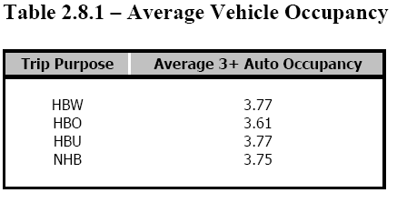
Mode split and auto occupancy analysis can be two separate steps or can be combined into a single step, depending on how a forecasting process is set up. In the simplest application a highway/transit split is made first which is followed by a split of automobile trips into auto driver and auto passenger trips. More complex analysis splits trips into multiple categories (single occupant auto, two person car pool, 3-5 person car pool, van pool, local bus, express bus, etc.). Auto occupancy analysis is often a highly simplified process which uses fixed auto occupancy rates for a given trip purpose or for given household size and auto ownership categories. This means that the forecasts of car pooling are insensitive to changes in the cost of travel, the cost of parking, the presence of special programs to promote car pooling, etc.
Assumptions: Some of the assumptions in mode choice analysis are as follows:
Choice only affected by time and cost characteristics. An important thing to understand about mode choice analysis is that shifts mode usage would only be predicted to occur only if there are changes in the characteristics of the modes, i.e. there must be a change in the in-vehicle time, out-of-vehicle time or cost of the automobile or transit for the model to predict changes in demand. Thus if one adds a lot of amenities to transit or substitutes a light rail transit system for a bus system without changes in travel times or costs, the model would not show any difference in demand, unless a ‘mode specific constant’ were used. People are assumed to make travel choices based only on the factors in the model. Factors not in the model will have no effect on results predicted by the models.
Omitted factors. Factors which are not included in the model such as crime, safety, security, etc. concerns have no effect. They are assumed to be included as a result of the calibration process. However, if an alternative has different characteristics for some of the omitted factors, no change will be predicted by the model. Such effects need to be done by hand and require considerable skill and assumptions.
Access times are simplified. No consideration is given to the ease of walking in a community and the characteristics of a waiting facility in the choice process. Strategies to improve local access to transit or the quality of a place to wait do not have an effect on the models.
Time and cost can be added. The disutility calculations assume that a traveler considers time and cost separately and mentally adds them up to determine their best choice for a trip.
Constant weights. The importance of time cost and convenience is assumed to remain constant for a given trip purpose. Trip purpose categories are very broad (i.e. 'shop', 'other'). Differences within these categories of the importance of time and cost are ignored.
Once trips have been split into highway and transit trips, the specific path that they use to travel from their origin to their destination must be found. These trips are then assigned to that path in the step called traffic assignment.
Traffic assignment is the most time consuming and data intensive step in the process and is done differently for highway trips and transit trips. The process first involves the calculation of the shortest path from each origin to all destinations (usually the minimum time path is used). Trips for each O-D pair are then assigned to the links in the minimum path and the trips are added up for each link. The assigned trip volume is then compared to the capacity of the link to see if it is congested. If a link is congested the speed on the link needs to be reduced to result in a larger travel time on that link. When speeds and travel times are changed the shortest path may change. Hence the whole process must be repeated many times (iterated) until there is an equilibrium between travel demand and travel supply. Trips on congested links will be shifted to uncongested links until this equilibrium, condition occurs.
There are a variety of ways in which the calculations are done to reach network equilibrium, in order to keep the computer time to a minimum. One way to get a feel for the accuracy of the models is to look at the resulting speeds on the network. These should be realistic after equilibrium.
Transit trip assignment is done in a similar way except that transit headways are adjusted rather than travel times. Transit headways (minutes between vehicles) affect the capacity of a transit route. Low headways mean that there is more frequent service and a greater number of vehicles. Transit supply and demand are also recalculated to reach an equilibrium between supply and demand.
It is important to understand the concept of equilibrium. If a highway or transit route is congested during the peak hour, its excess trips will be shifted to alternative routes. If the alternative routes are also congested the final results will show congestion over a wide part of the network. In the real world this congestion will eventually dissipate over time.
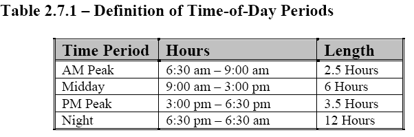
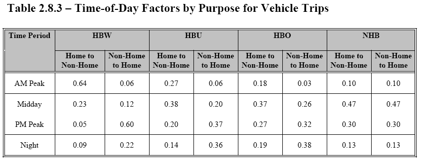
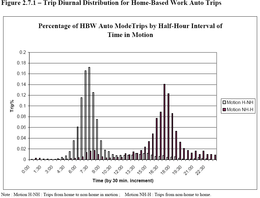
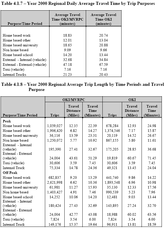
Another important step in assignment is the time of day analysis. Daily trip patterns need to be converted to peak time period traffic. A key assumption needed is the portion of daily travel that occurs during the peak period. This is normally used as a constant and conventional travel models have very limited capability to describe how travelers will shift their trips to less congested times of the day.
Assumptions and limitations: Some of the assumptions in traffic assignment are as follows:
Delay occurs on links. Most traffic assignment procedures assume that delay occurs on the links rather than at intersections. This is a good assumption for through roads and freeways but not for highways with extensive signalized intersections. Intersections involve highly complex movements and signal systems. Intersections are highly simplified in traffic if the assignment process does not modify control systems in reaching an equilibrium. Use of sophisticated traffic signal systems or enhanced network control of traffic cannot be analyzed with conventional traffic assignment procedures.
Travel only occurs on the network. It is assumed that all trips begin and end at a single point in a zone (the centroids) and occurs only on the links included in the network. Not all roads streets are included in the network nor all possible trip beginning and end points included. The zone/network system is a simplification of reality.
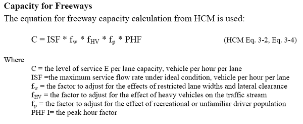
Capacities are simplified. To determine the capacity of roadways and transit systems requires a complex process of calculations that consider many factors. In most travel forecasts this is greatly simplified. Capacity is found based only on the number of lanes of a roadway and its type (freeway or arterial). Most travel demand models used for large transportation planning studies do not consider intersection capacity and the use of sophisticated traffic control systems in their calculations.
Time of day variations. Traffic varies considerably throughout the day and during the week. The travel demand forecasts are made on a daily basis for a typical weekday and then converted to peak hour conditions. Daily trips are multiplied by a "hour adjustment factor", for example 10%, to convert them to peak hour trips. The number assumed for this factor is very critical. A small variation, say plus or minus one percent, will make a large difference in the level of congestion that would be forecast on a network. Most models are unable to represent how travelers often cope with congestion by changine the time they make their trips.
Emphasis on peak hour travel. As described above, forecasts are done for the peak hour. A forecast for the peak hour of the day does not provide any information on what is happening the other 23 hours of the day. The duration of congestion beyond the peak hour is not determined. In addition travel forecasts are made for a 'average weekday'. Variations in travel by time of year or day of the week are usually not considered.
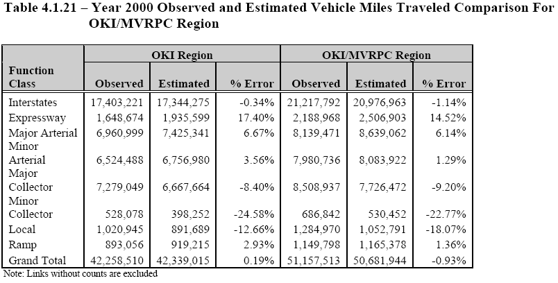
Equilibrium traffic assignment results indicate the amount of travel to be expected on each link in the network at some future date with a given transportation system. These link traffic volumes are the basic information that is used to determine a wide variety of effects of travel for plan evaluation. Some of the key effects are congestion, accidents, travel times, air pollution emissions. Each of these effects needs to be estimated through further calculations. Typically these are done by applying crash or emission rates by highway type and speed. Assumptions need to be made of the speed and characteristics of travel for non-peak hours of the day and for variation in travel by time of the year.
Specification
In this step, the model's mathematical form is specified (e.g., regression, cross classification, logit, lookup table) and the variables of interest are identified.
Estimation
In model estimation, one or more mathematical procedures are used to determine the likely values of the model parameters and coefficients. For example, when estimating the likely coefficient values for a logit model, the method of maximum likelihood estimation (MLE) is generally used. Empirically estimated models rely upon data, which is derived from surveys (e.g., Census, household travel surveys, air passenger surveys), traffic counts, or transit counts. Most estimation work is done with software packages such as SAS, SPSS, R, Stata, Alogit, LIMDEP/NLOGIT, or Biogeme.
Implementation
Once a model is estimated, it needs to be implemented so that it can be applied. Most travel models are implemented and applied using computer software. The TPB travel model makes use of software packages that are designed both specifically for travel demand forecasting (e.g., Cube Voyager and Cube Base) and more general software packages (e.g., Fortran, ArcGIS, Visual Basic).
Calibration/validation
Model calibration and validation generally occur in an iterative fashion. The model is validated in a "base year" against observed data to make sure that it is performing adequately and reasonably. Based on the performance of the model in model validation, small adjustments are made to the model ("model calibration") until the model accurately replicates observed patterns and behavior. Ideally, the model is validated to a different set of observed data than was used for model estimation. A "future year" validation can also be performed. Although there are no observed data for a future year, one can make sure that the model forecasts are reasonable and consistent with expectations. All travel models are validated against observed data.
Application
In the final step of the process, models are applied, generally using computer software, so that they may be used for developing forecasts.
In the broadest sense, a regional travel demand model consist of three elements:
Input Data
The two basic inputs to a regional travel demand model are
Output Data
Agencies performing such modeling traditionally follow a four-step planning process. In general terms, four-step travel demand models include the following stages:
The four-step model bases trip generation, trip distribution, and mode choice on socioeconomic and land-use data within the model area. Advanced versions of four-step models may also consider characteristics of the transportation network (such as tolls, parking costs, roadway capacity, or transit availability), and may include joint effects through feedback between the steps.
Four-step models consider the time-of-day in different ways. Many basic models simply use a 24-hour period and calculate daily trips, using an hourly capacity of the individual links to establish general capacity restraint across the net works. Others model peak periods or peak hours to better simulate actual network conditions and associated travel delays. In most cases, time-of-day factors are used to calculate either hourly, peak period, or daily volumes. Regardless, the time of day does not significantly affect whether the trip is made, but simply how it is assigned to the network.
Source: Metropolitan Washington Council of Government
The four-step model is a trip-based model that is used, in one form or another, by the majority of Metropolitan Planning Organizations (MPOs) that perform regional travel demand modeling.The first three steps of a trip-based travel model are used to estimate the demand for travel. In the fourth step, trip assignment, the travel demand is equilibrated with the travel supply, as trips are loaded onto one or more transportation networks. The geographic unit of analysis in a four-step model is the transportation analysis zone (TAZ). Usually an urban area is divided into hundreds or thousands of transportation analysis zones.
Advantages
Four-step models offer a proven and relatively simple approach to forecasting general travel demand, which in turn explains their prevalence. The relationships between the steps are clear and the data requirements relatively manageable; however, this relative simplicity does not necessarily reflect the actual complexity of travel behavior.
Disadvantages
Critics of four-step modeling practice believe that there are fundamental flaws associated with it that can only be rectified by implementing activity-based models. A summary of these concerns is documented in TRB Special Report 288: Metropolitan Travel Forecasting – Current Practice and Future Direction (SR 288) which argues that four step models often cannot effectively support analyses of contemporary policy concerns such as induced demand , alternative land use policies, vehicle emissions, freight movement, and non-motorized travel.
As noted in SR 288, four step models are not “behavioral in nature.” Rather they rely on statistical correlations between demographics and traffic patterns. Often, those correlations represent averages over long time periods, or broad areas. The result is that four-step models have difficulty reflecting small scale changes, dynamic effects, and changes in travel behavior that represent complex trade-offs of cost, convenience a nd time-savings under various constraints. Certain specific policy areas are identified in SR 288 as particularly difficult to represent in a four- step framework, including:
In an activity based model, travel is derived from participation in activities and depends on the organization of those activities. Travel patterns are organized within activity-based models as sets of r elated trips known as “tours”.
The socioeconomic characteristics of individual households are developed from survey data and other data sources, and are used to estimate household interactions and resulting travel patterns at a highly disaggregated level. The resulting model results can be aggregated in diverse ways to explore travel behavior in detail.
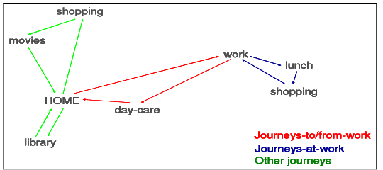
Activity- based models analyze travel in sets called “tours” that have a coordinated structure. Tours are made up of multiple trips that are anchored at important starting and ending points, such as home or work.
Source: An Overview of Tour-Based Models, presentation made by PB at Southeast Florida FSUTMS User’s Group Meeting, November 2007
In this example, which shows four tours that an individual might make in a single day, one tour (in blue) starts at work and is made up of trips from work to lunch, lunch to shopping, and shopping to work, while another tour (in red) is made up of a trip from home to work, from work to day-care, and from day-care to home. The other two tours (in green) are tours made for entertainment (home to shopping, shopping to movies, movies to home) and personal utility (home to library and library to home).
One of the benefits of estimating tours rather than trips is that coordinated decisions within a household may be modeled comprehensively based on a wider set of influential factors. Thus, for example, the home-to-library tour might be taken as a separate tour as shown in Figure 2.1. But in another household with different vehicle availability and socio-economic characteristics, or with different accessibility to possible destinations, the library activity could become a stop along with shopping and movies, or a stop on the home-to-work tour, or perhaps not take place at all. Activity-based models will situate trips in tours based on the likelihood of the various possibilities given detailed socio-economic, land use and network characteristics.
In order to create tours, activity-based models typically synthesize a set of persons and households that are distributed based on the socioeconomic and demographic characteristics of the study area. While similar processes have been used in cross-classification trip-generation models within the four-step framework (where zonal population characteristics are disaggregated into more specific categories), using a population synthesizer permits the model to build consistent marginal distributions of a much wider range of population characteristics. Population synthesis also allows the model to propagate (and re-aggregate) these characteristics at later stages in the model, and to explore subtle travel effects such as the decision not to make a certain tour based on the experienced level of highway congestion that are more difficult to accommodate in the four-step framework.
Using synthesized population data, the activity-based model estimates tours (or trip patterns) using the specific socioeconomic details of the household along with time of day constraints, accessibility indicators, available modes of travel, and other factors. Once created, these activity patterns are used to establish the primary and secondary destinations of the trips within each tour. Compared to typical four-step models, an activity-based model expands the patterns observed in an origin destination survey to the entire model region, and recognizes more of the details of those patterns in constructing future travel estimates.
BENEFITS OF ACTIVITY-BASED MODELS
As noted above in the discussion of four-step models, certain transportation policy questions are difficult to address in a standard four-step framework. However, TRB Special Report 288 also notes that “there is no single approach to travel forecasting or set of procedures that is ‘correct’ for all applications or all MPOs.” The report recommends
Development and implementation of new modeling approaches to demand forecasting that are better suited to providing reliable information for such applications as multimodal investment analyses, operational analyses, environmental assessments, evaluations of a wide range of policy alternatives, toll- facility revenue forecasts, and freight forecasts, and to meeting federal and state regulatory requirements.
Theoretical Benefits
Detail – Whereas most conventional four-step models base their forecasts on aggregate socioeconomic attributes of a transportation analysis zone (TAZ), activity-based models attempt, through various statistical strategies, to construct more detailed population distributions from available zonal data. Typically, to support this higher level of detail, activity-based models use much more highly disaggregate input data than four-step models, and often rely on parcel-based data to develop both residential and employment characteristics. Because activity-based models track person-level travel through the modeling process up to trip assignment, they support considerably more sensitive estimates of how various factors interact to influence overall trip- making.
Precision – In principle, the results of an activity-based model can also be examined at a very fine scale (down to the level of a household), although the statistical validity of such results is limited by the precision and variance of the input data. In addition, the impact of various policies on specific types of households can be examined explicitly at any point in the process, rather than attempting to recover those effects from aggregate results. Thus, for example, it would be just as easy to report statistics related to the travel impacts of increased tolls on households in a certain poor neighborhood as it would be to generate regional VMT estimates for all travelers. While some precision increase can be accomplished in four-step models using disaggregate data in the trip generation step, four-step models summarize that input to trip tables early in the process, losing considerable detail about the disaggregate impact of later steps in the modeling process such as trip distribution and mode choice.
Consistency – By virtue of their structure, activity-based models certainly create the opportunity to enforce greater consistency by requiring, for example, that tours begin and end at the same location, such as the home or work place. Further, activity-based models allow direct modeling of how trips destined to primary destinations, such as work or school, are related to trips to secondary destinations such as shopping or recreation. Activity-based models can also more easily capture the interaction of departure times and the sequencing of trips, as well as the consistency of mode choice during the course of a tour, all of which are necessary in modeling time- and congestion-based phenomena such as peak spreading and trip suppression (where travelers choose not to make a trip because congestion or other factors make it too inconvenient).
Behavioral Realism – It is sometimes claimed that activity-based models represent travel behavior more realistically than trip-based four-step models. This claim comes in two forms, practical and theoretical. At a practical level, activity-based models may provide better sensitivity to various inputs and express more accurate statistical relationships between various input factors and modeled outcomes. The models thus may produce forecasts that more closely resemble what would actually take place were the model’s input scenario to occur in reality. Unfortunately, there is little concrete evidence presently available to substantiate this claim, though interesting practical research is underway, most notably a project sponsored by Ohio DOT to compare an activity-based model and its advanced four-step counterpart in Columbus (Anderson et al, 2009).
The more theoretical version of the behavioral realism claim stems from the assertion that activity-based models “simulate” behavior. Leaving aside the trivial sense in which all travel demand models attempt to simulate what would happen given certain new conditions, the claim that activity-based models simulate behavior has two main variants. First, activity-based models are commonly implemented as a set of discrete choice models and corresponding utility functions. From the perspective of rational choice theory, such models can be said to simulate behavior, because they are ostensibly analogous to actual behavioral processes. Such a claim is not well supported by psychological and econometric research, however (for an extensive discussion, see Friedman, 1996). Second, activity-based models often use statistical techniques such as drawing samples from an empirical distribution that are described as “simulation” due to the use of that term to characterize a method for estimating complex statistical models where an analytic solution is not available but the result could be “simulated” through numerical techniques (Train, 2003). However, the use of the term “simulation” in this sense does not actually make any claim regarding the realism of activity-based models.
Analytic Flexibility –Activity-based models, which present more consistent and detailed results and are sensitive to a wider range of inputs, create greater opportunities for testing policy alternatives or transportation demand management strategies. In this way, the model becomes a more comprehensive policy analysis tool, rather than a simply a traffic volume generator. Also, the household-based structure of activity-based models, as well as the desirability of using extremely disaggregate input data, allows these models to operate effectively in conjunction with land use forecasting models.
Practical Benefits
As noted earlier, there are five significant policy areas identified in TRB’s Special Report 288 in which major model improvements are required in order to provide effective policy support:
- Time chosen for travel
- Travel Behavior related to demand policies such as “road pricing, telecommuting programs, transit vouchers, and land use controls”
- Non-motorized Travel
- Time-Specific traffic volumes and speeds
- Freight and Commercial Vehicle Movements.
Each of these areas benefits to a greater or lesser extent from activity-based modeling strategies, as follows:
Time chosen for travel is often a complex function of intra-household demands such as transporting children to school, negotiating work schedules with limited vehicles, telecommuting, and limitations of transit availability. Fully capturing these joint dependencies in relation to time chosen for travel is likely to be much more straightforward in an activity-based framework.
Travel demand policies present a broad a wide range of possible modeling needs, some of which can be partially handled using advanced four-step techniques. In general, however, the level of specificity that activity-based models offer with respect to variations in acceptable travel cost trade-offs across the population makes these models particularly well suited to analyzing travel demand policies.
Non-motorized travel is a particularly thorny problem, since the environmental factors that affect such travel often occur on a very small scale. For example, the absence of a hundred feet of sidewalk along a major arterial can effectively eliminate pedestrian travel to nearby destinations, yet such environmental effects are extremely difficult to code into any type of travel demand model. To the extent that sufficiently detailed input information can be made available (and forecast), activity-based models may be more sensitive at a person-by-person level to non-motorized travel characteristics.
Modeling time-specific traffic volumes and speeds probably requires dynamic traffic assignment (DTA), but DTA may be more effective in the context of activity-based trip models, as those can more easily model the time of demand and thus incorporate phenomena such as peak spreading. DTA is also a desirable component for analyzing tolling strategies, and in particular, value pricing strategies where tolls vary over time with the level of congestion. However DTA can work within both the four-step and activity-based model frameworks.
Freight and commercial vehicle movements are not intrinsically easier to handle using activity-based models. In fact, existing activity-based models have almost exclusively modeled freight and commercial vehicles using the same techniques as four-step models. The limiting factors in freight modeling have more to do with the sparse availability of data, and with the absence of detailed knowledge about the factors that influence freight and commercial vehicle movements, than they do with the overall model framework.
Highway Link
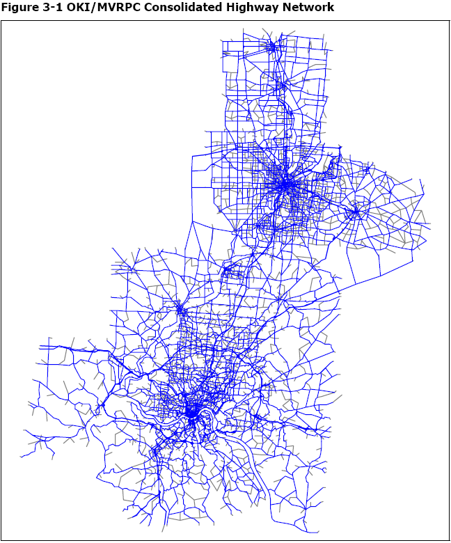
Highway Link Attributes
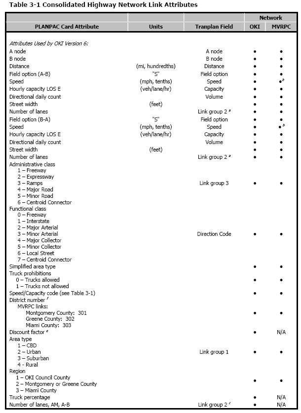
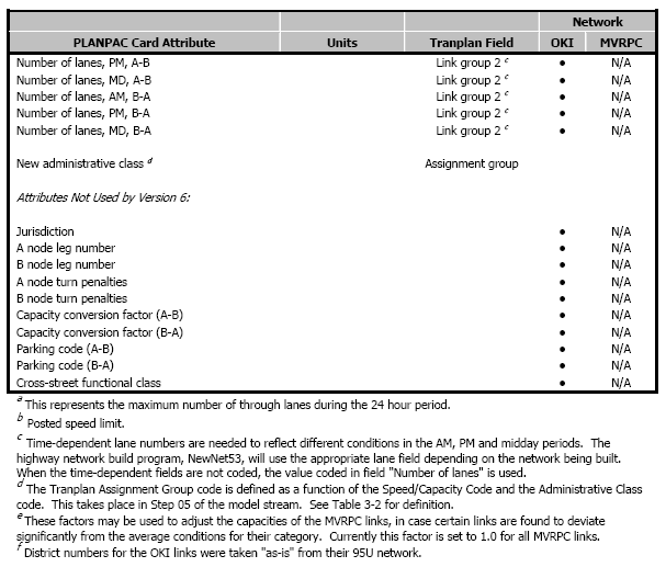
Speed/Capacity Lookup
Bus routes were assigned the following characteristics:
Hours of operation:
Traffic Analysis Zones (TAZs)
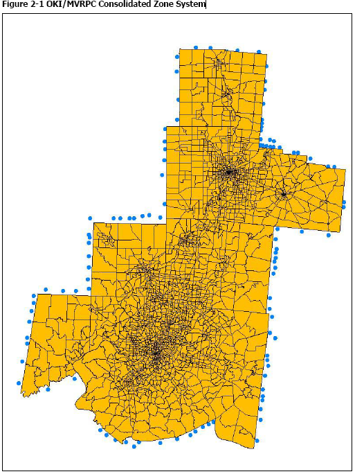
Each zone is assigned an area type designation as CBD, Urban, Suburban or Rural.
CBD - Predetermined downtown area.
Urban:
Suburban zones are zones not meeting the criteria for urban but have population densities 1.56 persons per acre. In some cases pockets of "suburbanization" have developed outside the primary central urban boundary or those of Hamilton or Middletown. Where two or more contiguous zones meeting urban criteria occur, the zones are designated suburban.
Rural zones are those which do not meet the criteria for CBD, urban or suburban as described above.
The consolidated model uses the following household classification variables:
OKI/MVRPC Travel Demand Model Validation Summary
Transportation models are being called upon to provide forecasts for a complex set of problems that in some cases can go beyond their capabilities and original purpose. Travel demand management, employer based trip reduction programs, pedestrian and bicycle programs, time of day shifts, changing age structure of the population and land use polices may not be handled well in the process.
Transportation travel forecasting models uses packaged computer programs which have limitations on how easily they can be changed. In some cases the models can be modified to accommodate additional factors or procedures (quick fix) while in other cases major modifications are needed or new software is required. The following are some potential modifications of the models that may help to improve their usefulness.
Better data. All models are based on data about travel patterns and behavior. If this data is out-of-date, incomplete or inaccurate the results will be poor no matter how good the models are. One of the most effective ways of improving model accuracy and value is to have a good basis of recent data that represent all components of the population to use to calibrate the models and to provide for checks of their accuracy. Models need to demonstrate that they provide an accurate picture of current travel before they should be used to forecast future travel.
Improve representation of bicycle and pedestrian travel. Travel by bicycle and by walking is not handled well in conventional travel demand models. Improved methods of dealing with these types of trips are needed. This can be done by incorporation of factors in trip generation models that relate trip making to pedestrian or bicycle amenities. Also methods of mode choice could be expanded to include these types of trips.
Better Auto Occupancy Models. Current auto occupancy procedures tend to be insensitive to a wide range of policies that may lead to more or less carpooling. Auto occupancy procedures need to be sensitive to the cost of parking and costs of travel as well as the number of trips that occur between an origin and destination. Also it may be desirable to treat ride sharing among family members differently that car pooling between persons from different households. Procedures that increase the number of trip purposes to deal with market segments that are likely to share rides could help with this problem.
Better time of day procedures. Levels of congestion in hours other than the peak period are needed to get a better understanding of the nature of congestion as it occurs throughout a day and over time into the future. Methods are needed to represent how travelers choose the time of travel, especially for non-work and non- school trips. Hourly conversion factors need to be looked at very carefully to insure that they represent actual variations in traffic.
Use more trip purposes. Additional trip purposes (market segments) may provide a way to get a better representation of complex household trip patterns and trip chaining. This would also provide trip generation procedures that are sensitive to more factors that would follow from travel management techniques.
Better representation of access. Land use policies that facilitate transit use or that provide high quality site design with good pedestrian access are not well represented in the transportation models. Improved methods are needed to measure the disutility of the access portion of transit and highway trips. Such methods would involve the calculation of an access index that was sensitive to the ease of access and waiting for transit vehicles in areas that used more transit/pedestrian/bicycle friendly design.
Incorporate costs into trip distribution. Trip distribution models should use a generalized measure of distance that includes costs of travel by different means including parking costs. Such models would then better show the sensitivity of travel patterns to cost changes.
Add Land Use Feedback. It is important to take steps to close the loop of the forecasting process to enable a better representation of the interaction of land use and travel demand. Land use simulation models should be added to the sequence of models to help to determine how a proposed transportation system will lead to land use changes.
Add intersection delays. In an urban traffic network most delay is encountered at traffic signals or stop signs rather than on the roads between intersections. Travel forecasting models should include routines that calculate the delay encountered at intersections. Moreover, intersection signal splits should be treated as a variable that would be modified as the traffic assignment process iterates to reach an equilibrium.